(still) nothing clever

And by this I mean uploading files from a PHP script to another HTTP URL, essentially submitting a web-form with a file-field from PHP. I needed this in Organik, it took me some hours to find out how. My hacky result is here for the world to reuse:

http://github.com/gromgull/randombits/blob/master/http_file_upload.php

Enjoy.

(updated 05/09/2011)

In the Organik project we’ve been using the noun-phrase extraction modules of OpenNLP toolkit to extract key concepts from text for doing Taxonomy Learning. OpenNLP comes with trained model files for English sentence detection, POS-tagging and either noun-phrase chunking or full parsing, and this works great.

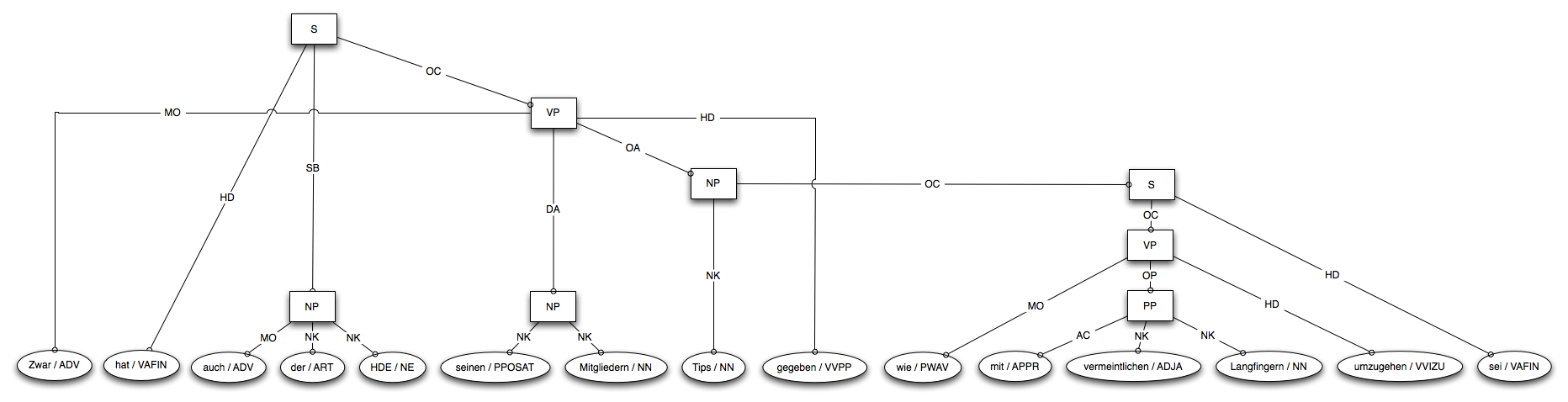
Of course in Organik we have some German partners who insist on using their awful german language [1] for everything – confusing us with their weird grammar. Finding a solution to this has been on my TODO list for about a year now. I had access to the Tiger Corpus of 50,000 German sentences marked up with POS-tags and syntactic structure. I have tried to use this for training a model for NP chunking, either using the OpenNLP MaxEnt model or with conditional random fields as implemented in FlexCRF. However, the models never performed better than around 60% precision and recall, and testing showed that this was really not enough. Returning to this problem now once again I have looked more closely at the input data, it turns out the syntactic structures used in the Tiger Corpus are quite detailed, containing far higher granularity of tag-types than what I need. For instance the structure for “Zwar hat auch der HDE seinen Mitgliedern Tips gegeben, wie mit vermeintlichen Langfingern umzugehen sei.” (click for readable picture):

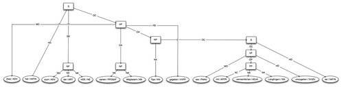
Here the entire “Tips […] wie mit vermeintlichen Langfingern umzugen sei”, is a noun-phrase. This (might) be linguistically correct, but it’s not very useful to me when I essentially want to do keyword extraction. Much more useful is the terms marked NK (Noun-Kernels), i.e. here “vermeintlichen Langfingern”. Another problem is that the tree is not continuous with regard to the original sentence, i.e. the word gegeben fits into the middle of the NP, but is not a part of it.

SO – I have preprocessed the entire corpus again, flattening the tree, taking the lowermost NK chain, or NP chunk as example. This gives me much shorter NPs in general, for which it is easier to learn a model AND the result is more useful in Organik. Running FlexCRF again on this data, splitting off a part of the data for testing, gives me a model with 94.03% F1-measure on the test data. This is quite comparable to what was achieved for English with FlexCRF in CRFChunker, for the WSJ corpus they report a F-Measure of 95%.

I cannot redistribute the corpus or training data, but here is the model as trained by FlexCRF for chunking: GermanNPChunkModel.tar.gz (17.7mb)

and for the POSTagging: GermanPOSTagModel.tar.gz (9.5mb)

Both are trained on 44,170 sentences, with about 900,000 words. The POSTagger was trained for 50 iterations, the Chunker for 100, both with 10% of the data used for testing.

In addition, here is a model file trained with OpenNLPs MaxEnt: OpenNLP_GermanChunk.bin.gz (5.2mb)

This was trained with the POS tags as generated by the German POStagger that ships with OpenNLP, and can be used with the OpenNLP tools like this:


java -cp $CP opennlp.tools.lang.german.SentenceDetector \
models/german/sentdetect/sentenceModel.bin.gz |
java -cp $CP opennlp.tools.lang.german.Tokenizer \
models/german/tokenizer/tokenModel.bin.gz |
java -cp $CP -Xmx100m opennlp.tools.lang.german.PosTagger \
models/german/postag/posModel.bin.gz |
java -cp $CP opennlp.tools.lang.english.TreebankChunker \
models/german/chunking/GermanChunk.bin.gz


That’s it. Let me know if you use it and it works for you!

Update 5/9/2011:
I have re-run the OpenNLP chunker with the most recent 1.5.1 version. The chunking model file format had changed, the updated file is here:
http://gromgull.net/2010/01/npchunking/OpenNLP_1.5.1-German-Chunker-TigerCorps07.zip. I did not redo the POS tagging, so if it changed from the old version the accuracy will suffer.

I’ve also put up the scripts I used to prepare this – starting with some corpus in the TIGER-XML treebank encoding format in tiger.xml and opennlp libraries in lib/:

# Convert XML to Flex
python tiger2flex.py tiger.xml > tiger.flex
# Reoplace POS tags with those OpenNLP produces
python retagflex.py tiger.flex > tiger.opennlp
# Learn chunking model
sh learnModel.sh tiger.opennlp chunkingmodel.zip

It’s a while since I wrote this code, so I am not 100% sure how it works any more, but it seems fine :)

[1] Completely unrelated, but to exercise your German parsing skills, check out some old newspaper articles. Die Zeit has their online archive available back to 1946, where you find sentence-gems like this: Zunächst waren wir geneigt, das geschaute Bild irgendwie umzurechnen auf materielle Werte, wir versuchten Arbeitskräfte und Zeit zu überschlagen, die nötig waren, um diese Wüste, die uns umgab, wieder neu gestalten zu können, herauszuführen aus diesem unfaßlichen Zustand der Zerstörung, überzuführen in eine Welt, die wir verstanden, in eine Welt,’ die uns bis dahin umgeben hatte. (ONE sentece!, from http://www.zeit.de/1946/01/Rueckkehr-nach-Deutschland)

From the I-will-never-actually-finish-this department I bring you the Semantic Web Cluster-ball:

I started this is a part of the Billion Triple Challenge work, it shows the how different sites on Semantic Web are linked together. The whole thing is an interactive SVG, I could not get it to embed here, so click on that image and mouse over things and be amazed. Clicking on the different predicates in the SVG will toggle showing that predicate, mouse over any link will show how many links are currently being shown. (NOTE: Only really tested in Firefox 3.5.X, it looked roughly ok in Chrome though.)

The data is extracted from the BTC triples by computing the Pay-Level-Domain (PLD, essentially the top-level domain, but with special rules for .co.uk domains and similar) for the subjects and objects, and if they differ, count the predicates that link them. I.e. a triple:

dbpedia:Albert_Einstein rdf:type foaf:Person.

would count as a link between http://dbpedia.org and http://xmlns.com for the rdf:type predicate. Counting all links like this gives us the top cross-domain linking predicates:

Most frequent is of course rdf:type, since most schemas are from different domains to the data, and most things have a type. The ball linked above is excluding type, since it’s not really a link. You can also see a version including rdf:type. The rest of the properties are more link-like, I am not sure what is going on with the akt:has-date though, anyone?

The visualisation idea is of course not mine, mainly I stole it from Chris Harrison: Wikipedia Clusterball. His is nicer since he has core nodes inside the ball. He points out that the “clustering” of nodes along the edge is important, as this brings out the structure of whatever is being mapped. My “clustering” method was very simple, I swap each node with the one giving me the largest decrease in edge distance, then repeat until the solution no longer improves. I couple this with a handful of random restarts and take the best solution. It’s essentially a greedy hill-climbing method, and I am sure it’s far from optimal, but it does at least something. For comparison, here is the ball on top without clustering applied.

The whole thing was of course hacked up in python, the javascript for the mouse-over etc. of the SVG uses prototype. I wanted to share the code, but it’s a horrible mess, and I’d rather not spend the time to clean it up. If you want it, drop me a line., see below. The data used to generate this is available either as a download: data.txt.gz (19Mb, 10,000 host-pairs and top 500 predicates), or a subset on Many Eyes (2,500 host-pairs and top 100 predicates, uploading 19Mb of data to Many Eyes crashed my Firefox :)

UPDATE: Richard Stirling asked for the code, so I spent 30 min cleaning it up a bit, grab it here: swball_code.tar.gz It includes the data+code needed to recreate the example above.

For completeness, Besbes is telling me to write up the final stats from the BTC data, for the object-part of the triples. I am afraid this data is quite dull, and there are not many interesting things to say, so it’ll be mostly tables. Enjoy :)

The BTC data contains 279,710,101 unique objects in total. Out of these:

• 90,007,431 appear more than once
• 7,995,747 more than 10 times
• 748,214 more than 100
• 43,479 more than 1,000
• 3,209 more than 10,000

The 280M objects are split into 162,764,271 resources and 116,945,830 literals. 13,538 of the resources are file:// URIs. The top 10 objects are:

Apart from the wikipedia link, all are types. No literals appear in the top 10 table. For the 116M unique literals we have 12,845,021 literals with a language tag and 2,067,768 with a datatype tag. The top 10 literals are:

I can’t be bothered to check it now, but I guess the  many Aye’s & Nay’s come from IRC chatlogs (#SWIG?).

Finally, I looked at the length of the literals used in the data, the longest literal is 65,244 unicode characters long (I wonder about this — this seems very close to 2¹⁶ bytes, some unicode characters with more than one byte, could it be truncated?). The distribution of literals/lenghts looks like this:

The most literals are around 10 characters in length, there is a peak for 19, which I seem to remember was caused by the standard time format (i.e. 2005-10-30T10:45UTC) being exactly 19 characters.

That’s it! I believe I now have published all my numbers on BTC :)

Know TvTropes.org? As pointed out by XKCD, a great place to lose hours of time reading about SoBadIt’sHorrible, HighOctaneNightmareFuel and thousands of other tropes, all with examples from comics, films, tv-series etc.

DFKI colleague Malte Kiesel has done the right thing and just released his linked open data wrapper for tvtropes, natuerally names dbTropes.org. Now go read about DiabolusExMachina, it will of course do content-negotiation so try it with your favourite RDF browser.

I helped too — I made the stylesheet and the “logo” :)

In Koble the auto-completion of thing-names used for wiki-editting, instant-search and adding relations  is getting slower and slower, mainly because I do:

result=[]
things=listAllThings()
for t in things:
   if t.startswith(key): res.append(t)
for t in things:
   if key in t: res.append(t)

Going through the list twice makes sure I get all things that match well first (i.e. the start with the string I complete for), and then things matching less well later (they only contain the string).

Of course the world has made up a far better data-structure for indexing prefix’es of string, namely the trie, or prefix tree. James Tauber had already implemented one in python, and kindly made it available. His version didn’t do everything I needed, so I added a few methods. Here is my updated version:

http://gromgull.net/2009/11/trie.py

Enjoy!

This is the fourth of my Billion Triple Challenge data-set statistics posts, if you only just got here, catch up on part I, II or  III.

I had these numbers ready for a long time, but never found the time to type it up as the it is not so exciting. However CaptSolo asked for it now to put in his very-soon-to-be-finished thesis, so I’ll hurry up. This is all about the classes used in the BTC data, i.e. the rdf:type triples.
Overall the data contains 143,293,758 type triples, assigning 283,815 different types to 104,562,695 different things.  For the types themselves:

• 213,281 types are used more than once
• 94,455 used more than 10
• 14,862 more than 100
• 1,730 more than 1000
• 288 more than 10000

If we take only these 288 top ones we cover 92% of all types triples, we can cover 90% of the typed things with only 105 types and over 50% of the data with only foaf:Person, sioc:WikiArticle, rss:Item and foaf:OnlineAccount. Out of all the “types” used 12,319 were BNodes, which is odd, but I guess possible, and 204 are literals, which is even odder. The top 10 types are:

Now for the things the types are assigned to, out of the 104,562,965 things with types, 52,865,376 are BNodes. If you pay attention you will now have realised that many things have more than one type assigned (143M type triples⇒104M things). In fact:

• 7,026,972 things have more than one type triple.
• 612,467 has more than 10
• 35,201 more than 100
• 1,025 more than 1,000
• 40 more than 10,000

Note I am talking here of type triples, i.e. the top 40 things may well have the same type assigned 10,000 times. The things having over 10,000 types assigned is a product of the partially inclusion of inferred triples in the data. For instance, for every context where RDFS inference has been applied, all properties will have rdf:type rdf:Property inferred. Looking at the number of unique types per thing shows that:

• 2,979,968 things have more than one type
• 78,208 have more than 10
• 4 more than 100

The 10 things with most unique types are all pretty boring:

Likewise the 10 things with the most types assigned, all product of materialised inferred triples:

That’s it — I hope it changed your life! :)

It’s all Cygri‘s fault — he encouraged me to add schema namespaces to the general areas on the semantic web cluster-tree. Now, again I misjudged horribly how long this was going to take. I thought the general idea was simple enough, I already had the data. One hour should do it. And now one full day later I have:

It’s the same map as last time, laid using graphviz’s neato as before. The heat-map of the properties was computed from the feature-vector of predicate counts, first I mapped all predicates to their “namespace”, by the slightly-dodgy-but-good-enough heuristic of taking the part of the URI before the last # or / character. Then I split the map into a grid of NxN points (I think I used N=30 in the end), and compute a new feature vector for each point. This vector is the sum of the mapped vector for each of the domains, divided by the distance. I.e. (if you prefer math) each point’s vector becomes:

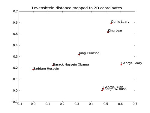
Where is the distance (here simple 2d euclidean), is each domain, is that domains position in the figure and is that domains feature vector. Normally it would be more natural to decrease the effect by the squared distance, but this gave less attractive results, and I ended up square-rooting it instead. The color is now simply on column of the resulting matrix normalised and mapped to a nice pylab colormap.

Now this was the fun and interesting part, and it took maybe 1 hour. As predicted. NOW, getting this plotted along with the nodes from the graph turned out to be a nightmare. Neato gave me the coordinates for the nodes, but would change them slightly when rendering to PNGs. Many hours of frustration later I ended up drawing all of it again with pylab, which worked really well. I would publish the code for this, but it’s so messy it makes grown men cry.

NOW I am off to analyse the result of the top-level domain interlinking on the billion triple data. The data-collection just finished running while I did this. … As he said.

So, not quite a billion triple challenge post, but the data is the same.  I had the idea that I compare the Pay-Level-Domains (PLD) of the context of the triples based on what predicates is used within each one. Then once I had the distance-metric, I could use FastMap to visualise it. It would be a quick hack, it would look smooth and great and be fun. In the end, many hours later, it wasn’t quick, the visual is not smooth (i.e. it doesn’t move) and I don’t know if it looks so great. It was fun though. Just go there and look at it:

As you can see it’s a large PNG with the new-and-exciting ImageMap technology used to position the info-popup, or rather used to activate the JavaScript used for the popups. I tried at first with SVG, but I couldn’t get SVG and XHTML and Javascript to play along, I guess in Firefox 5 it will work. The graph is laid out and generated Graphviz‘s neato, which also generated the imagemap.

So what do we actually see here? In short, a tree where domains that publish similar Semantic Web data are close to each other in the tree and have similar colours. In detail: I took the all PLDs that contained over 1,000 triples, this is around 7500, and counted the number of triples for each of the 500 most frequent predicates in the dataset. (These 500 predicates cover ≈94% of the data). This gave me a vector-space with 500 features for each of the PLDs, i.e. something like this:

Each value is the percentage of triples from this PLD that used this predicate. In this vector space I used the cosine-similarity to compute a distance matrix for all PLDs. With this distance matrix I thought I could apply FastMap, but it worked really badly and looked like this:

So instead of FastMap I used maketree from the complearn tools, this generates trees from a distance matrix, it generates very good results, but it is an iterative optimisation and it takes forever for large instances. Around this time I realised I wasn’t going to be able to visualise all 7500 PLDs, and cut it down to the 2000, 1000, 500, 100, 50 largest PLDs. Now this worked fine, but the result looked like a bog-standard graphviz graph, and it wasn’t very exciting (i.e not at all like this colourful thing). Now I realised that since I actually had numeric feature vectors in the first place I wasn’t restrained to using FastMap to make up coordinates, and I used PCA to map the input vector-space to a 3-dimensional space, normalised the values to [0;255] and used these as RGB values for colour. Ah – lovely pastel.

I think I underestimated the time this would take by at least a factor of 20. Oh well. Time for lunch.

This shows some strings positioned on a graph according to their Levenshtein string distance. (And let me note how appropriate it is that a man named Levenshtein should make a string distance algorithm)

The mapping from the distance matrix given by the string distance is then mapped to two dimensions using the FastMap algorithm by Christos Faloutsos and King-Ip Lin. This mapping can be also done with Multidimensional Scaling, (and I did so in my PhD work, I even claimed it was novel, but actually I was 40 years too late, oh well), but that algorithm is nasty and iterative. FastMap, as the name implies, is much faster, it doesn’t actually even need a full distance matrix (I think). It doesn’t always find the best solution, and it has a slight random element to it, so the solution might also vary each time it’s run, but it’s good enough for almost all cases. Again, I’ve implemented it in python – grab it here: fastmap.py

To get a feel for how it works, download the code, remove George Leary and see how it reverts to only one dimension for a sensible mapping.

The algorithm is straight-forward enough, for each dimension you want, repeat:

1. use a heuristic to find the two most distant points
2. the line between these two points becomes the first dimension, project all points to this line
3. recurse :)

The distance measure used keeps the projection “in mind”, so the second iteration will be different to the first.The whole thing is a bit like Principal Component Analysis, but without requiring an original matrix of feature vectors.

This is already quite old, from 1995, and I am sure something better exists now, but it’s a nice little thing to have in the toolbox. I wonder if it can be used to estimate numerical feature values for nominal attributes, in cases where all possible values are known?