Posts by gromgull.

Creating animations with graphviz

Here is a really pointless hack – Joern Hees asked me if I knew of any tools to force layout and visualise RDF graphs. We wondered about graphviz, but he wanted an interactive tool. When he left I wondered if it wouldn’t be quite easy to at least make an animation with graphviz. Of course it took longer than the 10 minutes, I expected, but it sort of worked. Based on the graphviz siblings example graph:

# get example
wget http://www.graphviz.org/Gallery/directed/siblings.gv.txt

# create the initial random layout
neato -Gstart=rand -Gmaxiter=1 -o i.dot siblings.gv.txt

# create 200 pngs for each iteration 
for x in $(seq 200) ; do neato -Gmaxiter=$x -Tpng -o $(printf "%03d" $x).png i.dot ; done

# resize so they are all the same size - graphviz sizing (-Gsize=4,4) is specified in inches and does not always produce PNGs of the same size.
for f in *.png ; do convert $f -resize 500x500! out.png ; mv out.png $f ; done

# make movie
mencoder mf://*.png -mf w=450:h=500:fps=10:type=png -ovc lavc -lavcopts vcodec=mpeg4:mbd=2:trell -oac copy -o output.avi

# upload to youtube
# profit!

(Of course there are many other tools that are much better than this – this is really a “because I can” case.)

A quick and dirty guide to YOUR first time with RDF

(This is written for the challenge from http://memespring.co.uk/2011/01/linked-data-rdfsparql-documentation-challenge/)

(To save you copy/pasting/typing you can download the examples from here: http://gromgull.net/2011/01/firstRDF/)

10 steps to make sense of RDF data:

  1. Install a debian or Ubuntu based system — I used Debian testing.
  2. Install rdflib and Berkely/Sleepycat DB by doing:
    sudo apt-get install python-rdflib python-bsddb3
    

    (I got rdflib version 2.4.2 – if you get version 3.X.X the code may look slightly different, let me know if you cannot work out the changes on your own)

  3. Find some data — I randomly picked the data behind the BIS Research Funding Explorer. You can find the raw RDF data on the source.data.gov.uk/data/ server. We will use the schema file from:

    http://source.data.gov.uk/data/research/bis-research-explorer/2010-03-04/research-schema.rdf

    and the education data from:

    http://source.data.gov.uk/data/education/bis-research-explorer/2010-03-04/education.data.gov.uk.nt

    We use the education data because it is smaller than the research data, only 500K vs 11M, and because there is a syntax error in the corresponding file for research :). In the same folders there are files called blahblah-void. These are statistics about the datasets, and we do not need them for this (see http://vocab.deri.ie/void/ for details).

  4. Load the data, type this into a python shell, or create a python file and run it:
    import rdflib
    
    g=rdflib.Graph('Sleepycat')
    g.open("db")
    
    g.load("http://source.data.gov.uk/data/education/bis-research-explorer/2010-03-04/education.data.gov.uk.nt", format='nt')
    g.load("http://source.data.gov.uk/data/research/bis-research-explorer/2010-03-04/research-schema.rdf")
    
    g.close()
    

    Note that the two files are in different RDF formats, both contain triples, but one is serialized as XML, the other in a ascii line-based format called N-Triples.You do not have to care about this, just tell rdflib to use the right parser with the format=X parameter, RDF/XML is the default.

  5. After the script has run there will be a new folder called db in the current directory, it contains the berkeley data-base files and indexes for the data. For the above example it’s about 1.5M
  6. Explore the data a bit, again type this into a python shell:
    • First open the DB again:
    • import rdflib
      g=rdflib.Graph('Sleepycat')
      g.open("db")
      len(g)
      
      -- Outputs: 3690 --
      

      The graph object is quite pythonic, and you can treat it like a collection of triples. Here len tells us we have loaded 3690 triples.

    • Find out what sorts of things this data describes. Things are typed by a triple with rdf:type as the predicate in RDF.
      for x in set(g.objects(None, rdflib.RDF.RDFNS["type"])): print x
      
      -- Outputs:
      http://www.w3.org/2002/07/owl#ObjectProperty
      http://www.w3.org/2002/07/owl#DatatypeProperty
      http://xmlns.com/foaf/0.1/Organization
      http://purl.org/vocab/aiiso/schema#Institution
      http://research.data.gov.uk/def/project/Location
      http://www.w3.org/1999/02/22-rdf-syntax-ns#Property
      http://www.w3.org/2000/01/rdf-schema#Class
      --
      

      rdflib gives you several handy functions that return python generators for doing simple triple based queries, here we used graph.objects, taking two parameters, the subjects and predicates to filter for, and returns a generator over all objects matching. rdflib also provides constants for the well-known RDF and RDFSchema vocabularies, we used this here to get the correct URI for the rdf:type predicate.

    • Now we know the data contains some Institutions, get a list using another rdflib triple-based query:
      for x in set(g.subjects(rdflib.RDF.RDFNS["type"], rdflib.URIRef('http://purl.org/vocab/aiiso/schema#Institution'))): print x
      
      -- Outputs:
      http://education.data.gov.uk/id/institution/UniversityOfWolverhampton
      http://education.data.gov.uk/id/institution/H-0081
      http://education.data.gov.uk/id/institution/H-0080
      ... (and many more) ...
      --
      

      This gives us a long list of all institutions. The set call here just iterates through the generator and removes duplicates.

    • Lets look at the triples about one in more detail:
      for t in g.triples((rdflib.URIRef('http://education.data.gov.uk/id/institution/UniversityColledgeOfLondon'), None, None)): print map(str,t)
      -- Outputs:
      ['http://education.data.gov.uk/id/institution/UniversityColledgeOfLondon', 'http://research.data.gov.uk/def/project/location', 'http://education.data.gov.uk/id/institution/UniversityColledgeOfLondon/WC1E6BT']
      ['http://education.data.gov.uk/id/institution/UniversityColledgeOfLondon', 'http://research.data.gov.uk/def/project/organisationName', 'University College London']
      ... (and many more) ...
      --
      

      This gives us a list of triples asserted about UCL, here we used the triples method of rdflib, it takes a single argument, a tuple representing the triple filters. The returned triples are also tuples, the map(str,t) just makes the output prettier.

  7. rdflib makes it very easy to work with triple based queries, but for more complex queries you quickly need SPARQL, this is also straight forward:
    PREFIX="""
    PREFIX owl: <http://www.w3.org/2002/07/owl#>
    PREFIX foaf: <http://xmlns.com/foaf/0.1/>
    PREFIX p: <http://research.data.gov.uk/def/project/>
    PREFIX aiiso: <http://purl.org/vocab/aiiso/schema#>
    PREFIX geo: <http://www.w3.org/2003/01/geo/wgs84_pos#>
    PREFIX skos: <http://www.w3.org/2004/02/skos/core#>
    PREFIX rdf: <http://www.w3.org/1999/02/22-rdf-syntax-ns#>
    PREFIX rdfs: <http://www.w3.org/2000/01/rdf-schema#>
    """
    
    list(g.query(PREFIX+"SELECT ?x ?label WHERE { ?x rdfs:label ?label ; a aiiso:Institution . } "))[:10]
    

    The prefixes defined here at the start lets us use short names instead of full URIs in the queries. The graph.query method returns a generator over tuples of variables bindings. This lists the first 10 – this is more or less the same as we did before, list all institutions, but this time also get the human readable label.

  8. Now a slightly more complicated example. Ask the knowledge base to find all institutions classified as public sector that took part in some project together:


    r=list(g.query(PREFIX+"""SELECT DISTINCT ?x ?xlabel ?y ?ylabel WHERE { 
       ?x rdfs:label ?xlabel ; 
          a aiiso:Institution ; 
          p:organisationSize 'Public Sector' ; 
          p:project ?p . 
    
       ?y rdfs:label ?ylabel ; 
          a aiiso:Institution ; 
          p:organisationSize 'Public Sector' ; 
          p:project ?p .
    
       FILTER (?x != ?y) } LIMIT 10 """))
    
    for x in r[:3]: print map(str,x)
    
    -- Outputs:
    ['http://education.data.gov.uk/id/institution/H-0155', 'Nottingham University', 'http://education.data.gov.uk/id/institution/H-0159', 'The University of Sheffield']
    ['http://education.data.gov.uk/id/institution/H-0155', 'University of Nottingham', 'http://education.data.gov.uk/id/institution/H-0159', 'University of Sheffield']
    ['http://education.data.gov.uk/id/institution/H-0159', 'Sheffield University', 'http://education.data.gov.uk/id/institution/H-0155', 'University of Nottingham']
    --
    

    All fairly straight forward, the FILTER is there to make sure the two institutions we find are not the same.
    (Disclaimer: there is a bug in rdflib (http://code.google.com/p/rdfextras/issues/detail?id=2) that makes this query take very long :( – it should be near instantaneous, but takes maybe 10 seconds for me. )

  9. The data we loaded so far do not have any details on the project that actually got funded, only the URI, for example: http://research.data.gov.uk/doc/project/tsb/100232. You can go there with your browser and find out that this is a project called “Nuclear transfer enhancement technology for bio processing and tissue engineering” – luckily so can rdflib, just call graph.load on the URI. Content-negotiation on the server will make sure that rdflib gets machine readable RDF when it asks. A for-loop over a rdflib triple query and loading all the project descriptions is left as an exercise to the reader :)
  10. That’s it! There are many places to go from here, just keep trying things out – if you get stuck try asking questions on http://www.semanticoverflow.com/ or in the IRC chatroom at irc://irc.freenode.net:6667/swig. Have fun!

Schema usage in the BTC2010 data

A little while back I spent about 1 CPU week computing which hosts use which namespaces in the BTC2010 data, i.e. I computed a matrix with hosts as rows, schemas as columns and each cell the number of triples using that namespace each host published. My plan was to use this to create a co-occurrence matrix for schemas, and then use this for computing similarities for hierarchical clustering. And I did. And it was not very amazing. Like Ed Summer’s neat LOD graph I wanted to use Protovis to make it pretty. Then, after making one version, uglier than the next I realised that just looking at the clustering tree as a javascript datastructure was just as useful, I gave up on the whole clustering thing.

Not wanting spent CPU hours go to waste, I instead coded up a direct view of the original matrix, getting a bit carried away I made a crappy non-animated, non-smooth version of Moritz Stefaner’s elastic lists using jquery-ui’s tablesorter plugin.

At http://gromgull.net/2010/10/btc/explore.html you can see the result. Clicking one a namespace will show only hosts publishing triples using this schema, and only schemas that co-occur with the one you picked. Conversely, click on a host will show the namespaces published by that host, and only hosts that use the same schemas (this makes less intuitive sense for hosts than for namespaces). You even get a little protovis histogram of the distribution of hosts/namespaces!

The usually caveats for the BTC data applies, i.e. this is a random sampling of parts of the semantic web, it doesn’t really mean anything :)

Redundancy in the BTC2010 Data, it’s only 1.4B triples!

In a comment here, Andreas Harth mentions that kaufkauf.net publishes the same triples in many contexts, and that this may skew the statistics a bit. As it turns out, not only kaufkauf.net is guilty of this, by stripping the fourth quad component of the data and removing duplicate triples the original 3,171,793,030 quads turn into “only” 1,441,499,718 triples.

36,123,031 triples occurred more than once in the data, 42 of these even more than 100,000 times. The top redundant triples are:

#triples subj pred obj
470,903 prot:A rdf:type prot:Chains
470,778 prot:A prot:Chain “A”^^<http://www.w3.org/2001/XMLSchema#string>
470,748 prot:A prot:ChainName “Chain A”^^<http://www.w3.org/2001/XMLSchema#string>
413,647 http://products.semweb.bestbuy.com/company.rdf#BusinessEntity_BestBuy rdf:type gr:BusinessEntity
366,073 foaf:Document rdfs:seeAlso http://dblp.l3s.de/d2r/sparql?query=DESCRIBE+%3Chttp://xmlns.com/foaf/0.1/Document%3E
361,900 dcmitype:Text rdfs:seeAlso http://dblp.l3s.de/d2r/sparql?query=DESCRIBE+%3Chttp://purl.org/dc/dcmitype/Text%3E
254,567 swrc:InProceedings rdfs:seeAlso http://dblp.l3s.de/d2r/sparql?query=DESCRIBE+%3Chttp://swrc.ontoware.org/ontology%23InProceedings%3E
184,530 foaf:Agent rdfs:seeAlso http://dblp.l3s.de/d2r/sparql?query=DESCRIBE+%3Chttp://xmlns.com/foaf/0.1/Agent%3E
159,627 http://www4.wiwiss.fu-berlin.de/flickrwrappr/ rdfs:label “flickr(tm) wrappr”@en
150,417 http://purl.org/obo/owl/OBO_REL#part_of rdf:type owl:ObjectProperty

This is all unfortunate, because I’ve been analysing the BTC data pretending that it’s a snapshot of the semantic web. Which perhaps it is? The data out there does of course look like this. Does the context of a triple change what it MEANS? If we had a trust/provenance stack in place I guess it would. Actually, I am not sure what this means for my statistics :)

At least I can now count the most common namespaces again, this time only from triples:

#triples namespace
651,432,324 http://data-gov.tw.rpi.edu/vocab/p/90
275,920,526 foaf
181,683,388 rdf
106,130,939 rdfs
34,959,224 dc11
33,289,653 http://purl.uniprot.org/core
16,674,480 gr
12,733,566 rss
12,368,342 dcterm
8,334,653 swrc

Compare to the numbers for quads, data-gov had exactly the same number of triples (no redundancy!), whereas rdf dropped from 588M to 181M, rdfs from 860M to 106M and GoodRelations from 527M to 16M. Looking at all namespaces, GoodRelations wins the most redundant award from 16% of all quads, to only 1.1% of all triples. Comparing change since 2009 still puts GoodRelations up high though, so no need for them to worry:

% change namespace
5579.997758 http://www.openlinksw.com/schema/attribution
4802.937827 http://www.openrdf.org/schema/serql
3969.768833 gr
2659.804256 urn:lsid:ubio.org:predicates:recordVersion
2655.011816 urn:lsid:ubio.org:predicates:lexicalStatus
2621.864105 urn:lsid:lsid.zoology.gla.ac.uk:predicates:mapping
2619.867255 urn:lsid:lsid.zoology.gla.ac.uk:predicates:rank
1539.092138 urn:lsid:ubio.org:predicates:hasCAVConcept
1063.282710 urn:lsid:lsid.zoology.gla.ac.uk:predicates:vernacularName
928.135900 http://spiele.j-crew.de/wiki/Spezial:URIResolver

And if I understood Kingsley Idehen correctly, there is something fishy about the attribution namespace from openlink as well, but I’ve done enough boring digging now.

Now I’m done doing boring counting – next time I hope I can have more fun visualisation, like Ed!!

SKOS Concepts in the BTC2010 data

Again Dan Brickley is making me work :) This time looking at the “hidden” schema that is SKOS concepts, (hidden because it is not really apparent when just looking at normal rdf:types). Dan suggested looking at topics used with FOAF, i.e. objects of foaf:topic, foaf:primaryTopic and foaf:interest triples, and also things used with Dublin Core subject (I used both http://purl.org/dc/elements/1.1/subject and http://purl.org/dc/terms/subject.

I found 1,136,475 unique FOAF topics in 8,119,528 triples, only 4,470 are bnodes, and only 265 (! i.e. only 0.002%) are literals. The top 10 topics are all of the type http://www.livejournal.com/interests.bml?int=??????, with varying number of ?s, this is obviously what people entered into the interest field of livejournal. More interesting are perhaps the top hosts:

#triples host
5,191,771 www.livejournal.com
1,819,836 www.deadjournal.com
771,439 www.vox.com
78,290 klab.lv
75,285 lj.rossia.org
70,380 lod.geospecies.org
18,398 my.opera.com
16,251 dbpedia.org
11,481 www.wasab.dk
9,815 wiki.sembase.at

So a lot of these topics are from FOAF exports of livejournal and friends. What I did not do, at least not yet, was to compare the list of FOAF topics with the things actually declared to be of type skos:Concept, this would be interesting.

Dublin Core looks quite different, it gives us 552,596 topics in 4,018,726 triples, but only 2,979 resources out of 921 are bnodes, the rest (i.e. 99.4%) are all literals.
The top 10 subjects according to DC are:

#triples subject
91,534 日記
38,566 写真
35,514 メル友募集
32,150 NAPLES
30,973 business
28,342 独り言
27,543 SoE Report
24,102 Congress
23,954 音楽
20,097

I do not even know what language most of these are (anyone?). Looking a bit further down the list, there are lots of government, education, crime, etc. Perhaps we can blame data.gov for this? I could have have kept track of the named-graphs these came from, but I didn’t. Maybe next time.

You can download the full raw counts for all subjects: FOAF topics (7.6mb), FOAF hosts and DC Topics (23mb).

BTC2009/2010 Raw Counts

Dan Brickley asked, so I put up the complete files with counts for predicates, namespaces, types, hosts, and pay-level domains here: http://gromgull.net/2010/09/btc2010data/.

Uploading them to manyeyes or similar would perhaps be more modern, but it was too much work :)

Aggregates over BTC2010 namespaces

Yesterday I dumped the most basic BTC2010 stats. Today I have processed them a bit more – and it gets slightly less boring.

First predicates, yesterday I had the raw count per predicate. Much more interesting is the namespaces the predicates are defined in. These are the top 10:

#triples namespace
860,532,348 rdfs
651,432,324 http://data-gov.tw.rpi.edu/vocab/p/90
588,063,466 rdf
527,347,381 gr
284,679,897 foaf
44,119,248 dc11
41,961,046 http://purl.uniprot.org/core
17,233,778 rss
13,661,605 http://www.proteinontology.info/po.owl
13,009,685 owl

(prefix abbreviations are made from prefix.cc \u2013 I am too lazy to fix the missing ones)

Now it gets interesting – because I did exactly this last year as well, and now we can compare!

Dropouts

In 2009 there were 3,817 different namespaces, this year we have 3,911, but actually only 2,945 occur in both. The biggest dropouts, i.e. namespaces that occurred last year, but not at all this year are:

#triples namespace
10,239,809 http://www.kisti.re.kr/isrl/ResearchRefOntology
5,443,549 nie
1,571,547 http://ontologycentral.com/2009/01/eurostat/ns
1,094,963 http://sindice.com/exfn/0.1
320,155 http://xmdr.org/ont/iso11179-3e3draft_r4.owl
307,534 http://cb.semsol.org/ns
242,427 nco
203,283 osag
187,600 http://auswiki.org/index.php/Special:URIResolver
159,536 nexif

I am of course shocked and saddened to see that the Nepomuk Information Elements ontology has fallen out of fashion all together, although it was a bit of a freak occurrence last year. I am not sure how we lost 10M research ontology triples?

Newcomers

Looking the other way around, what namespaces are new and popular this year, we get:

#triples namespace
651,432,324 http://data-gov.tw.rpi.edu/vocab/p/90
5,001,909 fec
2,689,813 http://transport.data.gov.uk/0/ontology/traffic
543,835 http://rdf.geospecies.org/ont/geospecies
526,304 http://data-gov.tw.rpi.edu/vocab/p/401
469,446 http://data-gov.tw.rpi.edu/2009/data-gov-twc.rdf
446,120 http://education.data.gov.uk/def/school
223,726 http://www.w3.org/TR/rdf-schema
190,890 http://wecowi.de/wiki/Spezial:URIResolver
166,511 http://data-gov.tw.rpi.edu/vocab/p/10

Here the introduction of data.gov and data.gov.uk were the big events last year.

Winners

For the namespaces that occurred both years we can find the biggest gainers. Here I calculated what ratio of the total triples each namespace constituted each year, and the increase in this ratio from 2009 to 2010. For example, GoodRelations, on top here, constituted nearly 16% of all triples in 2010, but only 2.91e-4% of all triples last year, for a cool increase of 570,000% :)

gain namespace
57058.38 gr
2636.34 http://www.openlinksw.com/schema/attribution
2182.81 http://www.openrdf.org/schema/serql
1944.68 http://www.w3.org/2007/OWL/testOntology
1235.02 http://referata.com/wiki/Special:URIResolver
1211.35 urn:lsid:ubio.org:predicates:recordVersion
1208.09 urn:lsid:ubio.org:predicates:lexicalStatus
1194.66 urn:lsid:lsid.zoology.gla.ac.uk:predicates:mapping
1191.39 urn:lsid:lsid.zoology.gla.ac.uk:predicates:rank
701.66 urn:lsid:ubio.org:predicates:hasCAVConcept

Losers

Similarly, we have the biggest losers, the ones who lost the most:

gain namespace
0.000185 http://purl.org/obo/metadata
0.000191 sioct
0.000380 vcard
0.000418 affy
0.000438 http://www.geneontology.org/go
0.000677 http://tap.stanford.edu/data
0.000719 urn://wymiwyg.org/knobot/default
0.000787 akts
0.000876 http://wymiwyg.org/ontologies/language-selection
0.000904 http://wymiwyg.org/ontologies/knobot

If your namespace is a loser, do not worry, remember that BTC is a more or less arbitrary snapshot of SOME semantic web data, and you can always catch up next year! :)

With a bit of luck I will do this again for the Pay-Level-Domains for the context URLs tomorrow.

Update

(a bit later)

You can get the full datasets for this from many eyes:

BTC2010 Basic stats

Another year, another billion triple dataset. This time it was released the same time my daughter was born, so running the stats script was delayed for a bit.

This year we’ve got a few more triples, perhaps making up for the fact that it wasn’t actually one billion last year :) we’ve now got 3.1B triples (or 3,171,793,030 if you want to be exact).

I’ve not had a chance to do anything really fun with this, so I’ll just dump the stats:

Subjects

  • 159,185,186 unique subjects
  • 147,663,612 occur in more than a single triple
  • 12,647,098 more than 10 times
  • 5,394,733 more 100
  • 313,493 more than 1,000
  • 46,116 more than 10,000
  • and 53 more than 100,000 times

For an average of 19.9252 per unique triple. Like last year, I am not sure if having more than 100,000 triples with the same subject really is useful for anyone?

Looking only at bnodes used as subjects we get:

  • 100,431,757 unique subjects
  • 98,744,109 occur in more than a single triple
  • 1,465,399 more than 10 times
  • 266,759 more 100
  • 4,956 more than 1,000
  • 48 more than 10,000

So 100M out of 159M subjects are bnodes, but they are used less often than the named resources.

The top subjects are as follows:

#triples subject
1,412,709 http://www.proteinontology.info/po.owl#A
895,776 http://openean.kaufkauf.net/id/
827,295 http://products.semweb.bestbuy.com/company.rdf#BusinessEntity_BestBuy
492,756 cycann:externalID
481,000 http://purl.uniprot.org/citations/15685292
445,430 foaf:Document
369,567 cycann:label
362,391 dcmitype:Text
357,309 http://sw.opencyc.org/concept/
349,988 http://purl.uniprot.org/citations/16973872

I do not know enough about the Proteine ontology to know why po:A is so popular. CYC we already had last year here, and I guess all products exposed by BestBuy have this URI as a subject.

Predicates

  • 95,379 unique predicates
  • 83,370 occur in more than one triples
  • 46,710 more than 10
  • 18,385 more than 100
  • 5,395 more than 1,000
  • 1,271 more than 10,000
  • 548 more than 100,000

The average predicate occurred in 33254.6 triples.

#triples predicate
557,268,190 rdf:type
384,891,996 rdfs:isDefinedBy
215,041,142 gr:hasGlobalLocationNumber
184,881,132 rdfs:label
175,141,343 rdfs:comment
168,719,459 gr:hasEAN_UCC-13
131,029,818 gr:hasManufacturer
112,635,203 rdfs:seeAlso
71,742,821 foaf:nick
71,036,882 foaf:knows

The usual suspects, rdf:type, comment, label, seeAlso and a bit of FOAF. New this year is lots of GoodRelations data!

Objects – Resources

Ignoring literals for the moment, looking only at resource-objects, we have:

  • 192,855,067 unique resources
  • 36,144,147 occur in more than a single triple
  • 2,905,294 more than 10 times
  • 197,052 more 100
  • 20,011 more than 1,000
  • 2,752 more than 10,000
  • and 370 more than 100,000 times

On average 7.72834 triples per object. This is both named objects and bnodes, looking at the bnodes only we get:

  • 97,617,548 unique resources
  • 616,825 occur in more than a single triple
  • 8,632 more than 10 times
  • 2,167 more 100
  • 1 more than 1,000

Since BNode IDs are only valid within a certain file it is limited how often then can appear, but still almost half the overall objects are bnodes.

The top ten bnode IDs are pretty boring, but the top 10 named resources are:

#triples resource-object
215,532,631 gr:BusinessEntity
215,153,113 ean:businessentities/
168,205,900 gr:ProductOrServiceModel
167,789,556 http://openean.kaufkauf.net/id/
71,051,459 foaf:Person
10,373,362 foaf:OnlineAccount
6,842,729 rss:item
6,025,094 rdf:Statement
4,647,293 foaf:Document
4,230,908 http://purl.uniprot.org/core/Resource

These are pretty much all types – compare to:

Types

A “type” being the object that occurs in a triple where rdf:type is the predicate gives us:

  • 170,020 types
  • 91,479 occur in more than a single triple
  • 20,196 more than 10 times
  • 4,325 more 100
  • 1,113 more than 1,000
  • 258 more than 10,000
  • and 89 more than 100,000 times

On average each type is used 3277.7 times, and the top 10 are:

#triples type
215,536,042 gr:BusinessEntity
168,208,826 gr:ProductOrServiceModel
71,520,943 foaf:Person
10,447,941 foaf:OnlineAccount
6,886,401 rss:item
6,066,069 rdf:Statement
4,674,162 foaf:Document
4,260,056 http://purl.uniprot.org/core/Resource
4,001,282 http://data-gov.tw.rpi.edu/2009/data-gov-twc.rdf#DataEntry
3,405,101 owl:Class

Not identical to the top resources, but quite similar. Lots of FOAF and new this year, lots of GoodRelations.

Contexts

Something changed with regard to context handling for BTC2010, this year we only have 8M contexts, last year we had over 35M.
I wonder if perhaps all of dbpedia is in one context this year?

  • 8,126,834 unique contexts
  • 8,048,574 occur in more than a single triple
  • 6,211,398 more than 10 times
  • 1,493,520 more 100
  • 321,466 more than 1,000
  • 61,360 more than 10,000
  • and 4799 more than 100,000 times

For an average of 389.958 triples per context. The 10 biggest contexts are:

#triples context
302,127 http://data-gov.tw.rpi.edu/raw/402/data-402.rdf
273,644 http://www.ling.helsinki.fi/kit/2004k/ctl310semw/WordNet/wordnet_nouns-20010201.rdf
259,824 http://static.cpantesters.org/author/M/MIYAGAWA.rss
207,513 http://data-gov.tw.rpi.edu/raw/401/data-401.rdf
193,944 http://static.cpantesters.org/author/D/DROLSKY.rss
189,528 http://static.cpantesters.org/author/S/SMUELLER.rss
170,899 http://data-gov.tw.rpi.edu/raw/59/data-59.rdf
166,454 http://zaltys.net/ontology/AKTiveSAOntology.owl
166,454 http://www.zaltys.net/ontology/AKTiveSAOntology.owl
165,948 http://lsdis.cs.uga.edu/~satya/Satya/jan24.owl

This concludes my boring stats dump for BTC2010 for now. Some information on literals and hopefully some graphs will come soon! I also plan to look into how these stats changed from last year – so far I see much more GoodRelations, but there must be other fun changes!

Illustrating the kernel trick

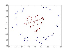
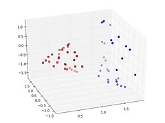
For a one paragraph intro to SVMs and the kernel-trick I wanted a a graphic that I’ve seen in a book (although forgotten where, perhaps in Pattern Classification?):

Simple idea — show some 2D data points that are not linearly separable, then transform to 3D somehow, and show that they are. I found nothing on google (at least nothing that was high enough resolution to reuse, so I wrote some lines of python with pylab and matplotlib:

import math
import pylab
import scipy

def vlen(v):
return math.sqrt(scipy.vdot(v,v))

p=scipy.randn(100,2)

a=scipy.array([x for x in p if vlen(x)>1.3 and vlen(x)<2])
b=scipy.array([x for x in p if vlen(x)<0.8])

pylab.scatter(a[:,0], a[:,1], s=30, c="blue")
pylab.scatter(b[:,0], b[:,1], s=50, c="red", marker='s')

pylab.savefig("linear.png")

fig = pylab.figure()
from mpl_toolkits.mplot3d import Axes3D
ax = Axes3D(fig)
ax.view_init(30,-110)

ax.scatter3D(map(vlen,a), a[:,0], a[:,1], s=30, c="blue")
ax.scatter3D(map(vlen,b), b[:,0], b[:,1], s=50, marker="s", c="red")

pylab.savefig("tranformed.png")

pylab.show()

Take — adapt — use for anything you like, you can rotate the 3D plot in the window that is shown and you can save the figures as PDF etc. Unfortunately, the sizing of markers in the 3d plot is not yet implemented in the latest matplotlib (0.99.1.2-3), so this only looks good with the latest SVN build.

The Machine Learning Algorithm with Capital A

A student came see me recently, wanting to do a Diplomarbeit (i.e. a MSc++) on a learning technique called Hierarchical Temporal Memory or HTMs. He had very specific ideas about what he wanted, and has already worked with the algorithm in his Projektarbeit (BSc++). I knew nothing about the approach, but remembered this reddit post, which was less than enthusiastic. I spoke to the student and read up on the thing a bit, and it seem interesting enough. It’s claimed to be close the way the brain learns/recognizes patterns and to be a general model of intelligence and  it will work for EVERYTHING. This reminded me of a few other things I’ve come across in the past years that claim to be the new Machine Learning algorithm with Capital A, i.e. the algorithm to end all other ML work, which will work on all problems, and so on. Here is a small collection of the three most interesting ones I remembered:

Hierarchical Temporal Models

HTMs are “invented” by Jeff Hawkin, whose track record includes making the Palm device and platform and later the Treo. Having your algorithm’s PR based on the celebrity status of the inventor is not really a good sign. The model is first presented in his book On Intelligence, which I’ve duly bought and am currently reading. The book is so far very interesting, although full of things like “[this is] how the brain actually works“, “Can we build intelligent machines? Yes. We can and we will.”, etc. As far as I understand, the model from the book was formally analysed and became the HTM algorithm in Dileep George‘s thesis: How the brain might work: A hierarchical and temporal model for learning and recognition. He applies to recognizing 32×32 pictures of various letters and objects.

The model is based on a hierarchy of sensing components, each dealing with a higher level of abstraction when processing input, the top of the hierarchy feeds into some traditional learning algorithm, such as a SVM for classification, or some clustering mechanism. In effect, the whole HTM is a form of feature pre-processing. The temporal aspect is introduces by the nodes observing their input (either the raw input, or their sub-nodes) over time, this (hopefully) gives rise to translation, rotation and  scale invariance, as the things you are watching move around.  I say watching here, because computer-vision seems to be the main application, although it’s of course applicable to EVERYTHING:

HTM technology has the potential to solve many difficult problems in machine learning, inference, and prediction. Some of the application areas we are exploring with our customers include recognizing objects in images, recognizing behaviors in videos, identifying the gender of a speaker, predicting traffic patterns, doing optical character recognition on messy text, evaluating medical images, and predicting click through patterns on the web.

The guys went on to make a company called Numenta for spreading this technique, they have a (not open-source, boo!) development framework you can play with.

Normalised Compression Distance

This beast goes under many names: compression based learning, compression-based dissimilarity measure, etc. The idea is in any case to reuse compression algorithms for learning, from good old DEFLATE algorithm from zip/gzip, to algorithms specific to some data-type, like DNA. The distance between things is then derived from how well they compress together with each other or with other data, and the distance metric can then be used for clustering, classification, anomaly detection, etc. The whole thing is supported by the theory of Kolmogorov Complexity and Minimum Description Length, i.e. it’s not just a hack.

I came across it back in 2003 in the Kuro5hin article Spam Filtering with gzip, back then I was very sceptical, thinking that any algorithm dedicated to doing classification MUST easily out-perform this. What I didn’t think about is that if you use the optimal compression for your data, then it finds all patterns in the data, and this is exactly what learning is about. Of course, gzip is pretty far from optimal, but it still works pretty well. I am not the only one who wasn’t convinced, this letter appeared in a physics journal in 2001, and led to some heated discussion: angry comment, angry reply, etc.

A bit later, I came across this again. Eamonn Keogh wrote Towards parameter-free data mining in 2004,  this paper makes a stronger case for this method being simple, easy and great and applicable to EVERYTHING:

[The Algorithm] can be implemented using any off-the-shelf compression algorithm with the addition of just a dozen or so lines of code. We will show that this approach is competitive or superior to the state-of-the-art approaches in anomaly/interestingness detection, classification, and clustering with empirical tests on time series/DNA/text/video datasets.

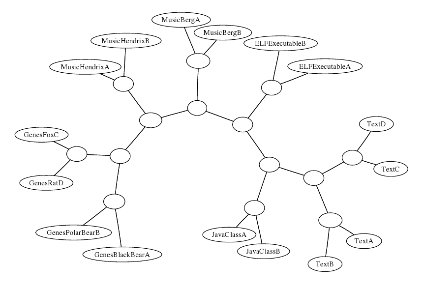
A bit later again I came across Rudi Cilibrasi (his page is broken atm.) thesis on Statistical Inference Through Data Compression. He has more examples, more theory and most importantly open-source software for everything: CompLearn (also down atm., but there are packages in debian). The method is very nice in that it makes no assumptions about the format of the input, i.e. no feature vectors or similar. Here is a clustering tree generated from a bunch of different files types:
Markov Logic Networks

I first came across Markov Logic Networks in the paper: Automatically Refining the Wikipedia Infobox Ontology. Here they have two intertwined problems they use machine learning to solve, firstly they want to map wikipedia category pages to WordNet Synsets, and secondly they want to arrange the wikipedia categories in a hierarhcy, i.e. by learning is-a relationships between categories. The solve the problem in two ways, the traditional way by using training a SVM to do the WordNet mappings, and using these mappings as an additional features for training a second SVM to do the is-a learning. This is all good, and works reasonably well, but by using Markov Logic Networks they can use joint inference to tackle both tasks at once. This is good since the two problems are clearly not independent, and now evidence that two categories are related can feed back and improve the probability that the map to WordNet synsets that are also related. Also, it allows different is-a relations to influence each other, i.e. if Gouda is-a Cheese is-a Food, then Gouda is probaby also a Food.

The software used in the paper is made by the people at the University of Washington, and is available as open-source: Alchemy – algorithms for statistical relational learning and probabilistic logic inference. The system combines logical and statistical AI, building on network structures much like Bayesian belief networks, in the end it’s a bit like Prolog programming, but with probabilities for all facts and relations, and these probabilities can be learned from data. For example, this cheerful example  about people dying of cancer, given this dependency network and some data about friends who influence each other to smoke and dying, you can estimate the probability that you smoke if your friend does and the probability that you will get cancer:

Since I am writing about it here, it is clear that this is applicable to EVERYTHING:

Markov logic serves as a general framework which can not only be used for the emerging field of statistical relational learning, but also can handle many classical machine learning tasks which many users are familiar with. […] Markov logic presents a language to handle machine learning problems intuitively and comprehensibly. […] We have applied it to link prediction, collective classification, entity resolution, social network analysis and other problems.

The others

Out of the three I think I find Markov Logic Network to be the most interesting, perhaps because it nicely bridges the symbolic and sub-symbolic AI worlds. This was my personal problem since I cannot readily dismiss symbolic AI as a Semantic Web person, but the more I read about about kernels, conditional random fields, online-learning using gradient descent etc. the more I realise that rule-learning and inductive logic programming probably isn’t going to catch up any time soon. NCD is a nice hack, but I tested it on clustering RDF resources, comparing the distance measure from my thesis with gzip’ping the RDF/XML or Turtle, and it did much worse. HTM still strikes me as a bit over-hyped, but I will of course be sorry when the bring the intelligent robots to market in 2011.

Some other learning frameworks that nearly made it into this post:

(wow – this got much longer than I intended)

http://www.idsia.ch/~juergen/